3 Elements of an R markdown file
3.1 YAML
The YAML is metadata for the document that goes right at the top of the file.
It can set the document author and title, the output format and many other things.
YAML format can be difficult to get right as it is sensitive to white space.
You can use an RStudio Addin from the package ymlthis to help write the YAML.
3.1.1 R code in YAML
It is possible to add R code to the YAML, for example to show the current date.
The R code needs to be enclosed in quote marks AND back-ticks with an r before the code.
If the code contains quotemarks, then they need to be different from the enclosing quotemarks (i.e. single vs double quotes).
---
title: "My Manuscript"
output: html_document
date: '`r format(Sys.Date(), "%d %B %Y")`'
---
See the data-time tutorial for more about the codes in "%d %B %Y".
3.1.2 Output formats
R markdown documents can be rendered in many different output formats, including
- presentations (with
xaringan::moon_readeror ioslides) - posters (with
posterdown) - books (with
bookdown). - theses (with
thesisdown)
This tutorial focuses on document-like reports.
There is a choice of output format for documents. This can be specified when the R markdown file is created in RStudio or by editing the YAML.
Producing an html file to view in a browser is the simplest, as nothing extra needs installing. The YAML should look something like this.
---
title: "My Manuscript"
output: html_document
---
Word documents are also easy; just change the output to word_document.
This can be very useful if you have a supervisor or collaborators who cannot cope with R markdown directly, but consider using the redoc package which lets you convert an edited word document back into R markdown.
Rendering the R markdown file as a PDF requires some external tools (LaTeX) to be installed (you don’t need to learn any LaTeX).
This can be done with the tinytxt package.
# run this only once
install.packages('tinytex')
tinytex::install_tinytex()
Then the output format in the YAML can be changed to pdf_document.
With PDF documents, it can be tricky to control exactly where the figures are positioned, so I recommend working with html as long as possible.
3.2 Text
Type to make text! RStudio has a built-in spell checker that will underline words it doesn’t recognise in red. Go to “Tools” >> “Global Options…” >> “Spelling” to change the language.
Paragraphs have a blank line between them. It is good practice to write one sentence per line. The extra line breaks will be removed when the document in knitted. If you want to force a line break, put two spaces at the end of the line.
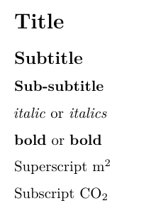
Formatting is generated with some special characters. For example:
# Title
## Subtitle
### Sub-subtitle
*italic* or _italics_
**bold** or __bold__
Superscript m^2^
Subscript CO~2~
If you actually want a #*_^~ in the text, you need to escape it by putting a backslash \ before it, e.g. \#.
If you don’t like formatting the document by hand, you can use the RStudio visual editor by clicking on the grey Å above the document.
A more complete list is given in the R markdown cheat sheet.
3.3 Code chunks
Code in an R markdown document is contained in code chunks.
This is a code chunk that loads the penguin data from the palmerpenguins package.
```{r import, echo = FALSE}
data(penguins, package = "palmerpenguins)
```
It starts with three back-ticks, followed by braces. Inside the braces, the “r” indicates that this is a chunk in the R language. The next word is the optional chunk name. After the comma are optional chunk arguments. Then on a new line is the body of the chunk. The chunk ends with three back-ticks on their own line.
3.3.1 Making a chunk
You can type the back-ticks and braces needed to make a chunk, but it is easier to get RStudio to insert the chunk. You can do this with the +C button or use the keyboard shortcut ctrl+alt+i (on a mac Command+Option+i ).
3.3.2 Chunk language
We will just work with R chunks, but it is possible to run chunks in other languages in RStudio, including Python.
3.3.3 Chunk names
It is a good idea to name chunks. If you don’t, they will automatically be called “unnamed-chunk-n” where “n” is a incrementing number. This is inconvenient for debugging (you need to work out which chunk is “unnamed-chunk-37”) and for working with any image files generated by the document. In section 6 you will see how to use chunk names to cross-reference figures and tables in your document.
3.3.4 Chunk options
There are lots of chunk options, but only a few that you will need to use frequently. Here are some and their default.
-
echo(TRUE) Show the chunk’s code in the output. -
eval(TRUE) Run the chunk code. -
include(TRUE) Include the output of the chunk in the document. -
message(TRUE) Include messages from R. -
warning(TRUE) Include warnings from R. -
error(FALSE) If TRUE, shows any error message. If FALSE, stops knitting when there is an error in R code.
I leave message and warning as TRUE while I am writing the document, so I can see any possible problems, and set them to FALSE when I knit the final version.
I sometimes find it useful to set error to TRUE as can make it easier to debug any errors in the code.
Chunk options for figures are shown in section 4.1.1.
Full list http://yihui.name/knitr/options/
3.3.5 Setting default chunk options
Default chunk options can be set for all chunks with knitr::opts_chunk$set in the first chunk.
New R markdown files created by RStudio automatically have this in a chunk called “setup.”
```{r setup, include=FALSE}
knitr::opts_chunk$set(echo = TRUE)
```
This chunk sets echo = TRUE for all chunks.
The include=FALSE will stop any output from this chunk being included in the output.
3.3.6 Running a chunk
Code in chunks will be run when the document is knitted (unless eval = FALSE), but it is also useful to run the code interactively to check that it works.
You can do this by clicking on the green play buttons at the right of the chunk (Fig. 3.1) or from the Run button above the document.
If the code depends on previous chunks, the grey/green icon will run them all.
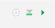
Figure 3.1: The green run chunk icon and the grey/green icon to run all previous chunks.
3.3.7 Hiding a chunk
If a chunk has a lot of code, it can be useful to hide it to make it easier to navigate the document. The grey arrow next to the line numbers will do this. Sections of text can also be hidden.
3.3.8 Environments and working directory
R knits R markdown documents in a new R session. The environment is empty: the R markdown document does not have access to any objects in your current environment (this is a good thing for reproducible analyses). This means that any data you want to use in the document needs to be imported by the code in the document.
The working directory for the new R session used when knitting the R markdown file is the directory where the file is.
If the file is in the root directory of an RStudio project, relative paths will work the same way in the R markdown document as from the console.
If the file is in a sub-directory, use here::here() to form paths relative to the project root.
Exercise
Download file https://raw.githubusercontent.com/biostats-r/biostats/main/Rmarkdown/data/Florida-precip.csv and save it into your RStudio project folder. The file gives monthly precipitation data from Florida, Bergen since 1983, extracted from https://seklima.met.no/. Earlier data are available from a weather station on Nordnes. Make an R chunk in your R markdown document and use it to import the file into R.
Hint
- Re-read the importing data chapter of the working in R book.
- Check the delimiter and decimal separator.
- Make sure the Rmarkdown document loads tidyverse.
Change the column headers so they are easier to work with.
Hint
See Working in R book section on non-standard names for suggestions on what names are good.
- Use the
col_namesargument toread_delim()(remember to skip the old column names) - OR use
rename(new_name = `Old Name`) - OR use
janitor::clean_names()
Convert the date column to date format
Hint
- Use the
col_typesargument toread_delim() - OR use
lubridate::dmy()(check help file to see thetruncatedargument)
3.4 Inline code
In addition to the output from chunks of code, you can insert code directly into text.
Inline code is enclosed by back-ticks and starts with an r.
Seven times six is `r 7 * 6`Seven times six is 42
If you want numbers written as words, use the package english.
Seven times six is `r english::words(7 * 6)`Seven times six is forty-two
It is best to keep inline code short to keep the text readable. One trick is to do all necessary calculation in a previous chunk, so only the name of the object with the result needs to be in the inline code. If there are many results to report, consider storing them in a list as in the following example.
cor_adelie <- cor.test(
  ~ bill_length_mm + body_mass_g,
  data = penguins,
  subset = species == "Adelie")

adelie_list <- list(
  #degrees of freedom
  df = cor_adelie$parameter,
  # extract correlation and round
  est = round(cor_adelie$estimate, 2),
  #format p.value with an "=" is the first character is not "<".
  #See the characters tutorial for more on the stringr package and regular expressions.
  p_val = str_replace(
    string = format.pval(cor_adelie$p.value, eps = 0.001),
    pattern = "^(?!<)",
    replacement = "= ")
)
Bill length and body mass in Adelie penguins are positively correlated,
r = `r adelie_list$est` (df = `r adelie_list$df`, p `r adelie_list$p_val`).Bill length and body mass in Adelie penguins are positively correlated, r = 0.55 (df = 149, p < 0.001).