8 Working with multiple tables in dplyr
All the dplyr functions we have looked at so far work on a single data frame.
This chapter introduces joins, which work on a pair of data frames with at least one identifying variable in common, and the bind_* functions which bind two or more data frames together.
8.1 Merging data frames with mutating joins
Mutating joins combine two data frames by matching rows according to one or more identifying variables that are in both data frames.
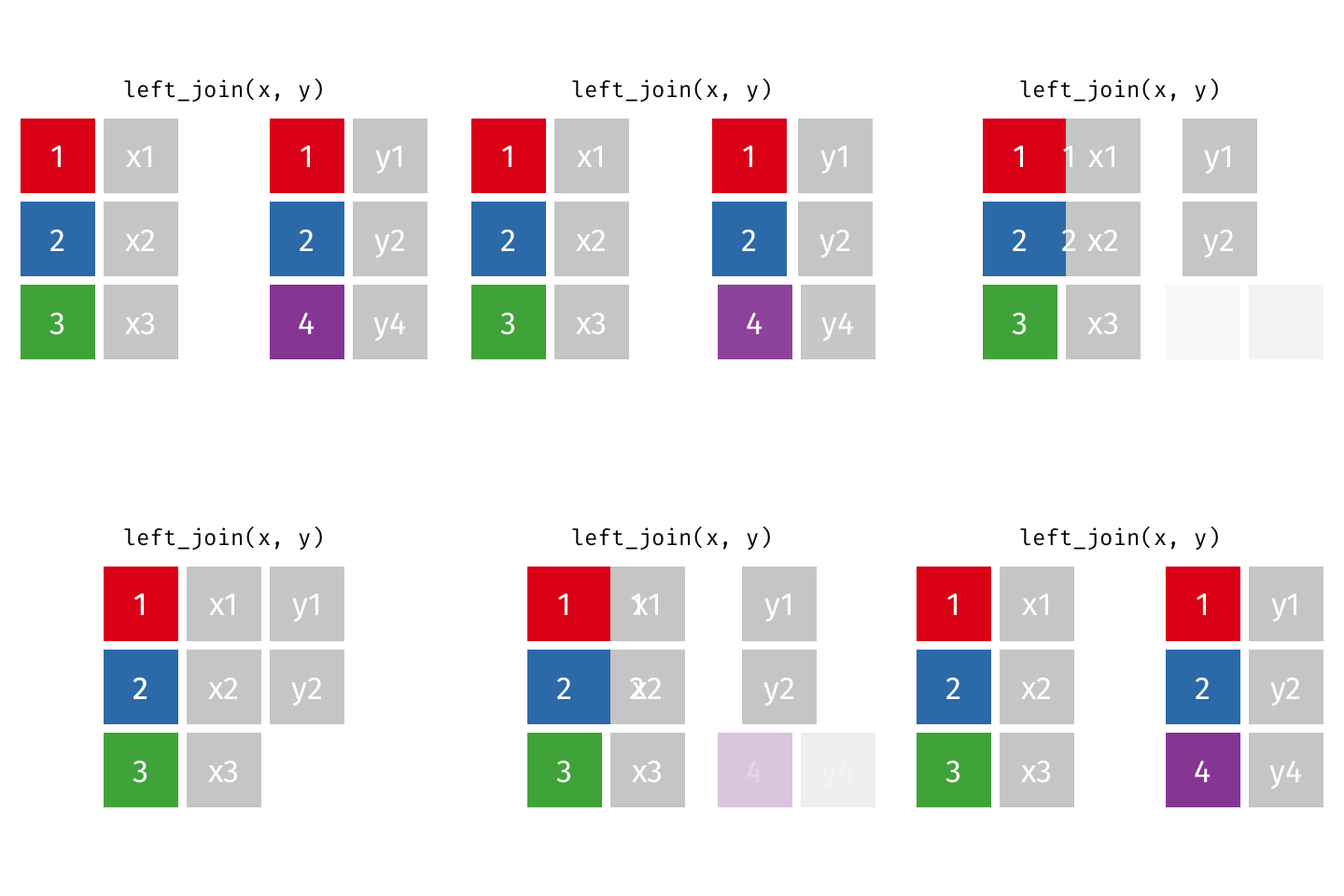
The most commonly used mutating join is a left join. Left joins take all rows from the first data set, and the rows from the second data frame where the values of the identifying variable match the first (Fig. 8.1).

Figure 8.1: Left join. The coloured column contains the identifiers.
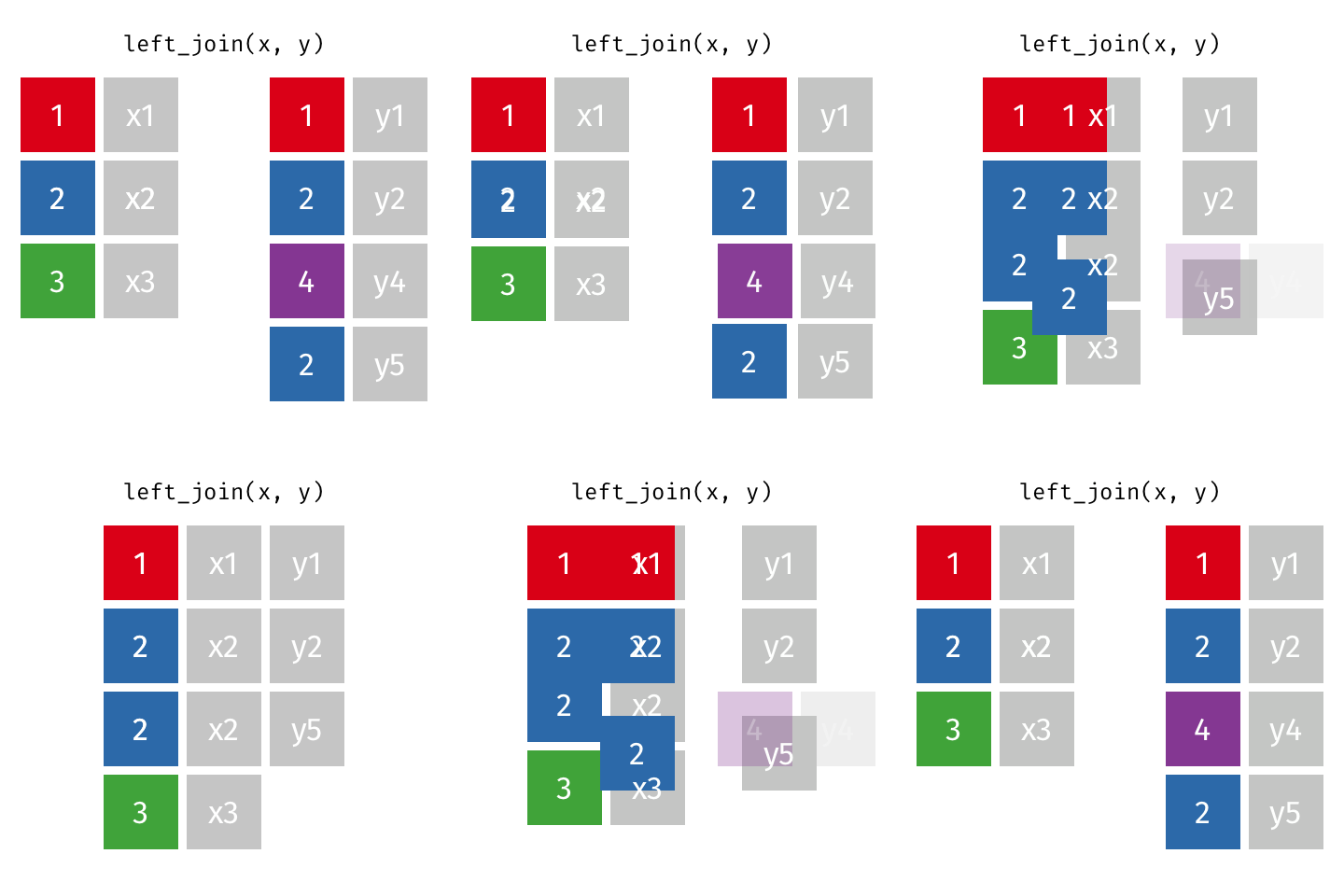
If there are duplicate values in the identifying column, this (Fig. 8.2) causes the matching rows to be duplicated. If the number of rows in the result increases when you were not expecting it, that can indicate that your identifier are not unique.

Figure 8.2: Left join. The coloured column contains the identifiers.
Left joins are implemented in dplyr with left_join().
Let use left_join() to add the location of each island to the penguin data set.
# location of the three islands in the Palmer Archipelago

penguin_islands <- tribble(
  ~ island, ~ Latitude, ~ Longitude, # tribble is a convenient way to make small datasets
  "Torgersen", -64.766667,-64.083333,
  "Biscoe", -64.818569, -63.775636,
  #"Dream",  -64.733333, -64.233333, # Dream data missing
  "Alpha", -64.316667, -63)

penguin_islands
## # A tibble: 3 × 3
## island Latitude Longitude
## <chr> <dbl> <dbl>
## 1 Torgersen -64.8 -64.1
## 2 Biscoe -64.8 -63.8
## 3 Alpha -64.3 -63The first two arguments to left_join() are the data frames, the third is the by argument which tells the join which column to make the join by.
Here, we are joining by a single column with the same name in both data frames.
It is possible to join by multiple columns and where the columns have different names in each dataset.
penguin_small <- penguins |>
  group_by(species) |>
  slice(1:2) # small version of data for easy viewing


left_join(penguin_small, penguin_islands, by = "island")
## # A tibble: 6 × 10
## # Groups: species [3]
## species island bill_length_mm bill_depth_mm flipper_length_… body_mass_g sex
## <fct> <chr> <dbl> <dbl> <int> <int> <fct>
## 1 Adelie Torge… 39.1 18.7 181 3750 male
## 2 Adelie Torge… 39.5 17.4 186 3800 fema…
## 3 Chinst… Dream 46.5 17.9 192 3500 fema…
## 4 Chinst… Dream 50 19.5 196 3900 male
## 5 Gentoo Biscoe 46.1 13.2 211 4500 fema…
## 6 Gentoo Biscoe 50 16.3 230 5700 male
## # … with 3 more variables: year <int>, Latitude <dbl>, Longitude <dbl>Only three of the four islands in penguin_islands have data in the penguins data set.
Different variants of mutating joins will treat this in different ways.
-
left_join()takes all rows from the first (left) data frame and matching rows from the second (right). -
right_join()does the opposite toleft_join(), taking all rows from the second (right) data frame and matching rows from the first. -
inner_join()will take only rows that match in both data frames. -
full_join()will take all rows from in both data frames.
In all cases, missing values will are given an NA.
8.2 All possible combinations
The mutating joins described above give you the rows from each data frame where the identifying variables match.
Sometimes you want all possible combinations of rows.
This is known as the Cartesian product and can be generated with crosing().
crosing() works with data frames as well as vectors as shown here.
crossing(a = letters[1:3], b = 1:2)## # A tibble: 6 × 2
## a b
## <chr> <int>
## 1 a 1
## 2 a 2
## 3 b 1
## 4 b 2
## 5 c 1
## 6 c 28.3 Filtering joins
Filtering joins let you filter one dataset according to whether rows have a match in the a second dataset.
semi_join() finds rows that have a matching row

Figure 8.3: Left join. The coloured column contains the identifiers.
penguin_islands |>
  semi_join(penguins, by = "island")
## # A tibble: 2 × 3
## island Latitude Longitude
## <chr> <dbl> <dbl>
## 1 Torgersen -64.8 -64.1
## 2 Biscoe -64.8 -63.8anti_join() finds rows that do not have a matching row

Figure 8.4: Left join. The coloured column contains the identifiers.
penguin_islands |>
  anti_join(penguins, by = "island")
## # A tibble: 1 × 3
## island Latitude Longitude
## <chr> <dbl> <dbl>
## 1 Alpha -64.3 -63These can be very useful when cleaning data to find problems.
8.4 Binding data frames together
If we have two or more data frames that we want to combine we can one of the bind_* functions.
8.4.1 More columns - bind_cols()
If the data frames contain information about the same observations, they can be combined with bind_cols().
So data1, data2, and data3 can be combined to make one data frame with many columns
bind_cols(data1, data2, data3)bind_cols() expects that the row order is the same in both datasets, but cannot check this.
It only checks that the number of rows is the same in each data frame.
If possible, use a join instead.
8.4.2 More rows - bind_rows()
If the data frame contain more observations (rows), and typically at least some of the same columns, they can be combined with bind_rows().
This is useful if, for example, there are data from two years that need combining.
One feature of bind_rows() that I find useful is the .id argument that makes an extra column for an identifier.
svalbard_islands <-  tribble( ~ island, ~ Latitude, ~ Longitude,
   "Nordaustlandet", 79.558405, 24.017351,
 "Prins Karls Forland", 78.554090, 11.256545)

bind_rows(
  Palmer = penguin_islands,
  Svalbard = svalbard_islands,
  .id = "Archipelago")
## # A tibble: 5 × 4
## Archipelago island Latitude Longitude
## <chr> <chr> <dbl> <dbl>
## 1 Palmer Torgersen -64.8 -64.1
## 2 Palmer Biscoe -64.8 -63.8
## 3 Palmer Alpha -64.3 -63
## 4 Svalbard Nordaustlandet 79.6 24.0
## 5 Svalbard Prins Karls Forland 78.6 11.3